Summary of Orbits Explained

Orbits Explained is a novel approach to understanding planetary orbits and how the Laws of Isaac Newton and Johannes Kepler apply. This webpage contains a synopsis of the chapters presented in Orbits Explained. Proofs in this synopsis are presented using logic and easy math but the proofs are abbreviated to allow fluid reading. A more detailed presentation of all the steps of easy math is available for those interested in the book Orbits Explained which is available for purchase on the Amazon website by clicking the link http://amazon.com/dp/B0DP1YLH3B. This overview begins with some elementary vector instruction to give the pure beginner the confidence to follow this short and convenient synopsis of Orbits Explained. In other words, – “Welcome, everyone.”

( You can return to the homepage of Orbits Explained by clicking here. )

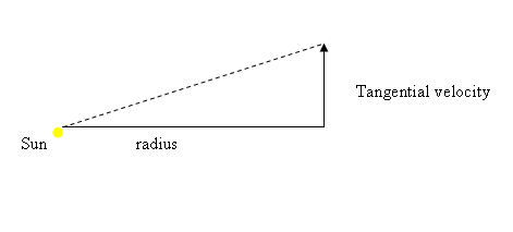
Let’s start with an explanation of vectors. Below is a diagram of a planet orbiting the Sun.

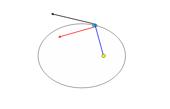
In the drawing above, a planet drawn in blue is orbiting the Sun drawn in yellow. We will call the imaginary straight line to the Sun, the “distance radius” or at times simply the “radius”. It is represented by the solid blue line. The actual direction and speed of the planet are indicated by the black arrow. The black arrow in the diagram is an example of a velocity vector. A velocity vector is an arrow whose length and orientation represent the speed and direction, respectively, of travel. The black arrow represents the total velocity of the planet and lies on a line that is the tangent to the orbit. The tangent is defined to be the line that grazes the curve of the orbit, touching it at only one point, without crossing the curve of the orbit. The red arrow represents a different aspect of the velocity; it relates to the speed of the planet which is measured solely in the direction that is at a right angle to the distance radius to the Sun. This velocity is known as tangential velocity. (Do not be confused by terminology. The tangential velocity of the blue planet is not along the tangent line to the orbit. The total velocity of the planet represented by the black arrow is tangent to the orbit). Tangential velocity (red arrow) and distance to the Sun (blue line) are of prime concern to us throughout our proofs in Orbits Explained. As is true of all vectors, the length of a velocity vector arrow can be adjusted so that it represents the velocity of the planet. A planet moving slower than another will have a velocity vector arrow that is shorter than the velocity vector arrow of a faster moving planet.

Let’s state a few things about the time it takes for one trip around an orbit.

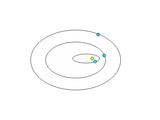
     In the drawing above, there are several planets orbiting the Sun. Each orbit differs in size from the others. Planets in the larger orbits take more time to complete one orbit. The time it takes to orbit once around the Sun is known as the period.

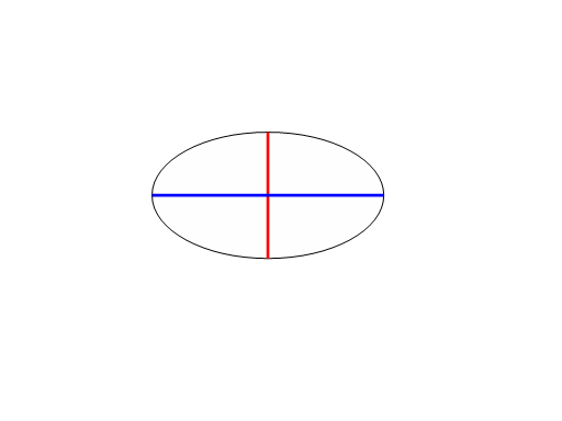
Let’s define the 2 basic dimensions of orbits. In the drawing below, the longest dimension of an orbit is the major axis. It is drawn in blue. Half the distance of the major axis is referred to as the semimajor axis. The minor axis is drawn in red.

     Now let’s look at historical laws that apply to planetary orbits. Kepler’s Three Planetary Law’s describe the fundamental behavior of planets. These Laws are based on Johannes Kepler’s brilliant analysis of Tycho Brahe’s empirical astronomical observations of planets’ movements across the sky.

     A special feature of Orbits Explained is that it proves Kepler’s Three Planetary Laws and Newton’s Inverse Square Law of Force without using any astronomical observations or other empirical data. In other words, these laws are proven in “a priori” fashion. You will see proofs of the following aspects of orbits:

1. Planets travel in elliptical orbits. This is Kepler’s First Planetary Law.
2. Planets sweep out equal areas in equal times. This is Kepler’s Second Planetary Law. Newton explained this in a priori fashion. We will add his a priori proof to our own set of a priori proofs in Orbits Explained.
3. Planets’ periods are proportional to the square root of the cube of their semimajor axis.  This is Kepler’s Third Planetary Law.
4. The gravitational force on a planet decreases with the square of the distance to the Sun. This is Newton’s Inverse Square Law of Force.
5. Throughout its orbit a planet lacks a constant amount of energy that it would need to gain in order to escape from the Sun.  I refer to this as the Energy Equation. It could also referred to as the Law of Planetary Capture.

As proofs of these five laws are demonstrated, it will become evident that they are fundamentally interrelated.

All of the five planetary laws mentioned above will be derived in novel fashion by introducing an original mathematical device called the hododyne. Another name for the hododyne is the Inverse Proportion Machine. It will be described superficially in this overview. The formal geometric and algebraic proofs for the hododyne are found in Chapters 8 and 9 of the full text of Orbits Explained.  The hododyne can be visualized as an immense template, larger than the orbit itself, engine-like, regulating the path and the speed of the planet.  Specifically, the hododyne is responsible for compelling the planet to behave with a given speed and direction in accordance with what is proper for the planet’s position with respect to the Sun.

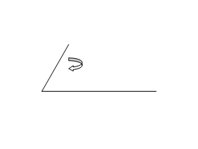
Remarkably, the hododyne is simply a line that is bent so that the resulting two parts can be made to spin around each other:

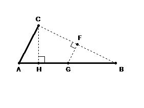
     How can something so apparently simple explain something as complex as an orbit?  The answer lies in the act of assigning landmarks to the parts of the hododyne. One of the landmarks will represent the position of the Sun. Another will represent the position of the planet. Other landmarks will simply be geometrical locations on the spinning parts of the hododyne.  Specifically, we create landmarks of the hododyne by first connecting the far ends of the bent parts by a straight line CB in the diagram below; then perpendicular lines HC and GF are drawn at specified locations.

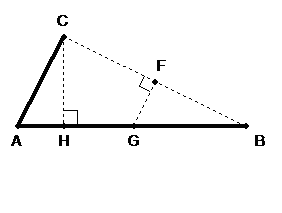
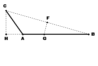
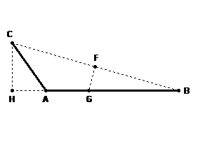
  In the hododyne above, AC and AB are the two spinning parts of the hododyne.  The point F bisects the connecting line CB. Segments FG and HC are created so that they are perpendicular to segments CB and AB respectively.  When necessary, the segment AB is given an extension so that a perpendicular can be drawn to meet point C as has been done in the arrangement below:

Chapter 9 of the full text of Orbits Explained contains the mathematical proof that for a hododyne as labeled above, segment AG is inversely proportional to segment HB. In other words as the two parts of the hododyne spin, the lengths of these segments change; one grows while the other diminishes in such a fashion that their numerical product is a constant; the length of HB times the length of AG is a constant.

     The recognition of the intrinsic inverse proportion properties of the hododyne invites us to look for a behavioral match in nature which involves properties that are inversely proportional to each other. These suitable properties could be assigned to the segments of the hododyne that are inversely proportional to each other. Such a match does indeed exist for the planetary properties of distance to the Sun and tangential velocity.  The inverse proportion between distance to the Sun and tangential velocity is the root of the entire set of a priori proofs presented in Orbits Explained by using the hododyne. Let’s see why tangential velocity and distance to the Sun are inversely proportional. We’ll look at Isaac Newton’s work.

     In the course of proving that a planet’s radius to the Sun sweeps equal areas in equal times, Newton, in essence, simultaneously proved that tangential velocity is inversely proportional to distance to the Sun. So, let’s examine Newton’s a priori proof regarding equal areas swept in equal times. We will follow the general scheme of Newton’s Proof as presented in Feynman’s Lost Lecture, The Motion of Planets Around the Sun, by David Goodstein and Judith Goodstein, published by Norton Press.

     Newton’s diagram is reproduced below. In Chapter 5 of Orbits Explained, Newton’s proof and diagram will be analyzed in detail.  Briefly here, suppose that a body is in motion at a constant speed, not subject to gravity.

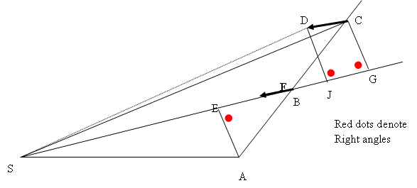
We are interested in the area swept by the line which connects the moving body to the point, S. Let the body move from A to B in a unit of time and then from B to C in an equal unit of time. Since its speed is constant, the distance AB will equal the distance BC. Now, employ a little geometry. Angle ABE is equal to angle CBG by the rules of intersecting lines. Angles AEB and BGC are right angles. Side AB is equal to side BC. Thus the right triangles AEB and BGC are equal since they both have the same three angles and the same length of hypotenuse. So, side GC is equal to side AE. The area of a triangle is equal to the base times the height divided by two. The area of triangle SAB is equal to the area of triangle SBC since they share a base SB and their heights, AE and GC, are equal. So, in the absence of gravity, as the object moves in equal times from A to B and then from B to C, the corresponding areas swept, SAB and SBC, are equal. Thus equal areas are swept in equal times in the absence of gravitational force.

     In Chapter 5 of Orbits Explained it will be shown, using similar triangles in Newton’s fashion, that in a gravitational field, the planet moves from B to D instead of from B to C. It will also be shown that the area swept will be SBD and that this area is equal to the area swept in the absence of gravity, area SBC.  In other words the gravitational force does not change the amount of area swept. And thus, even in the presence of gravity, equal areas are swept in equal times.

           We therefore see that Newton showed the following two statements to be true: As an object moves past a stationary position at constant speed, it sweeps out equal areas in equal times. If the moving object is subject to a force attracting it to a stationary position, the object will still sweep out equal areas in equal times.

Now let’s see how equal areas swept in equal times can be restated in terms of an inverse proportion so that we can apply inverse proportion properties to the hododyne’s segments HB and AG. As stated a few paragraphs above, the inverse proportion inherent in the phenomenon of equal areas swept in equal times relates two things to each other:

1. The distance to the Sun
2. The speed of the planet as measured along a line that is perpendicular to the direction towards the Sun. This particular aspect of speed is conventionally labeled the tangential velocity.

In the diagram below it will be shown that during a given small moment of time, the triangle of area swept by a planet is determined by its base which is the radius distance to the Sun, and its height which is determined by the tangential velocity of the planet.

The area of a triangle is equal to one half the base times its height. From that property it follows that any triangle whose base is caused to vary in inverse proportion to its height will have a constant area. Consider what happens to areas swept by the planet during successive equal tiny time intervals. During each equal instant of time the distance traveled by the planet in the direction of tangential velocity is directly proportional to the tangential velocity itself since the product of time and velocity is what determines distance. This distance traveled during the instant in time determines the height of the triangle of area swept by the planet. The other important side of the triangle, its base, represents the distance of the planet to the Sun, as was previously stated. Since in Orbits Explained we will be able to show that the triangular area swept by the planet during equal instants of time is constant, we can state that the height of the triangle (proportional to the planet’s tangential velocity) and the base of the triangle (equal to the planet’s distance to the Sun) must be inversely proportional to each other. Alas, we have our two inversely related properties, tangential velocity and distance to the Sun, to assign to the hododyne.

Let’s pause for a moment to note that a subtle and hidden logical choice was made in order to prove that equal areas are swept in equal times. We logically chose to use tangential velocity of the planet instead of total velocity of the planet to give us the “height” of the triangle of area swept. This is justifiable and logical because the total velocity of a planet can be broken into two components, one radial (along the line to the Sun) and one tangential (perpendicular to the line to the Sun). This concept is fully diagrammed and explored in Chapter 17 of the book Orbits Explained. In an instant of time the planet’s motion due to its radial component of velocity does not sweep any area at all since it is directly along the line connecting the planet to the Sun so it can logically be ignored.

Now we can pursue our plan of exploiting the inverse proportion between the planet’s momentary tangential velocity and the planet’s distance to the Sun by using our geometric device, the hododyne, to generate line segments that are inversely proportional to each other. All that needs to be done is to assign one line segment to represent distance to the Sun and the other line segment to represent tangential velocity of the planet during an instant of time. Then as the two parts of the hododyne are made to spin, the position and tangential velocity of the planet become evident, revealing the orbital path of the planet as follows:

First, let’s recall that as the parts of the hododyne spin, the angle between the parts might be less than or greater than 90 degrees and that Point H moves to an extension of line AB when the angle between the spinning segments AC and AB is greater than 90 degrees:

For either positional arrangement, the segment HB can be assigned to represent tangential velocity during an instant in time. The segment AG can be assigned to represent the radius distance to the Sun. These two assignments are justifiable since, as stated above, these two segments of the hododyne are inversely proportional to each other just as the radius distance to the Sun is inversely proportional to the tangential velocity of the planet in an instant of time.

Note in the diagram below that as the hododyne segment AB spins, the segment AB becomes the radius of a full circle that is traced by point B. The full circle that is traced contains what is known as the hodograph. It was described by Sir William Rowan Hamilton in 1846.

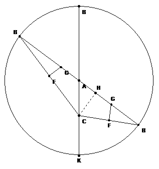
  In anticipation of being able to determine the position and tangential velocity of the planet, we can draw two representative positions of the hododyne on such a hodograph circle. One hododyne position, drawn on the left side of the circle, is arranged so that its segments AC and AB are less than 90 degrees from each other. The other hododyne position, on the right side of the circle, is arranged so that the angle between those segments is greater than 90 degrees:

 Let’s see why the hododyne diagram above proves that a planet is always on an elliptical curve:

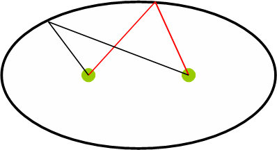
First, let’s note that by definition, a moving point lies on an ellipse if its distances from two other fixed points sum to a constant.  The two fixed points are called foci of the ellipse. For illustrative purposes we can restate this by example whereby the sum of the lengths of the red lines is the same as the sum of the lengths of the black lines in the ellipse above. Now let’s inspect the hodograph and hododyne:

Note that in the hodograph the line AB is the radius of the outer circle. Here is a hint about how we will proceed. We will let the line AB spin around point A so that point B traces a circle. We will examine what happens to triangles such as BFG and BCH as line AB spins. But before we take line AB for a spin, let’s look closely at the hododyne in our diagram. Since for any hododyne, point F is a bisector of the connecting segment CB, there are two similar triangles created, CFG and BFG, when we draw the extra dotted line CG. We will use those similar triangles to demonstrate that an ellipse will be traced once we let line AB spin, and that G, the planet’s position, is always on that ellipse and that A and C are the two foci of that ellipse. It is worthwhile to note that point A is the center of the hodograph circle and also represents the position of the Sun at one focus of the ellipse. Look at the line AB. It is of constant length since it is one of the line segments of the hododyne. Note that the length of CG added to the length AG must be equal to the length of AB since the length of CG is equal to the length of BG by the similar triangles, CFG and BFG, mentioned above. So BG + AG = BA = CG + GA. In other words CG + GA = a constant length equal to BA, the length of the spinning part of the hododyne. Now observe that C and A are fixed points since A is the bend between the parts of the hododyne and C is the end of one of the parts of the hododyne. By studying the diagram we can see that point G is on an ellipse since the sum of its distances, GA and CG to the fixed points A and C is a constant. Thus the planet at point G travels an elliptical path around the Sun as determined by the hododyne.

So, the hododyne has proved to us in a priori fashion that planets travel in elliptical orbits. In Orbits Explained we will use this proof to expand to proofs of other properties of a planet in orbit. Specifically, using stepwise methods, it will be shown in the full text of the book Orbits Explained that as the segment AB spins around segment AC, the following planetary properties can be seen in the hododyne and hodograph:

1. As the hododyne part AB spins around the hododyne part AC, the length of the segment AG represents the distance from the planet to the Sun.
2. Point A represents the position of the Sun. Point G represents the position of the planet.
3. The direction of the segment AG indicates the direction of the line that connects the planet to the Sun.
4. We will resolve a geometrical problem that arises from having our two inversely proportional line segments AG and BH on the same line. We will address the fact that the planet’s radius to the Sun, AG, and the planet’s tangential velocity, BH, can not be on the same line. They must by definition be at 90 degrees from each other. We will justify the statement that the line segments representing velocities are actually ninety degrees away from their true directions when we allow a hododyne to spin. This is the ninety degree correction rule for hododynes. This will justify the statement that the  true direction of tangential velocity is 90 degrees from segment HB.
5. Tangential velocity will be shown to only be a component of the total velocity of the planet. Total velocity of the planet will be shown in Orbits Explained to be represented by line segment CB in the hododyne. By applying the rules for components of vectors as they relate to the path of the planet and its tangential velocity, the following properties of total velocity become evident: We will justify assigning the direction of motion of the planet to be perpendicular to the direction of line segment CB in any instant of time. We will show that the length of the line segment CB indicates how fast the planet is traveling. We will distinguish in Orbits Explained  how line segment CB relates to the total velocity of the planet whereas line segment HB relates to tangential velocity, the specific component of total velocity of the planet that is at a right angle to the radius line to the Sun.
6. We will demonstrate in Orbits Explained that segment HC relates to the planet’s radial velocity. Radial velocity is the speed at which the planet travels along the imaginary line joining the planet to the Sun. Concerning the direction of radial velocity the ninety degree correction rule for velocity on the hododyne will be applied. We will distinguish in Orbits Explained how line segment CB relates to the total velocity of the planet whereas line segment HC relates to radial velocity, the specific component of total velocity of the planet that is along the radius line to the Sun. 

This is a good moment to examine our central claim that we can use the hododyne to prove in a priori fashion that planets travel in elliptical orbits. If true, then we also will have proved the inverse square law of force, which states that the attractive force between two bodies varies inversely with the square of the distance between them, because it can be mathematically derived by using the premise that orbits are elliptical. In the same manner, we will also have mathematically proved Kepler’s Third Law which regulates how much time passes during one orbit around the Sun. So, let’s examine our central claim. Isaac Newton proved in a priori fashion that a body moving past another sweeps out equal areas in equal times. He showed that this is true whether or not there was an attracting force between the two bodies. We strategically chose to point out that sweeping equal areas in equal times occurs when tangential velocity is inversely proportional to the distance to the Sun. We then chose those two properties to assign to the hododyne, the inverse proportion machine, to show that an ellipse would be traced by the path of the planet. But we must look at the arrangement of planet and Sun and the speed of the moving body before assessing our claim that we have a valid proof. For example, consider the body moving past a stationary body in the absence of any attractive force between them. The body sweeps out equal areas in equal times. The distance between the two bodies is inversely proportional to the tangential velocity of the moving body. If we apply the hododyne, it tells us that the moving body will travel in an elliptical orbit around the stationary body. The dilemma is that in the absence of attractive force the moving body will continue on its straight line path until infinity despite satisfying the condition that its distance to the stationary body is inversely proportional to its tangential velocity. The dilemma is resolved by noting that the hododyne is indeed a template that is applicable to stable repetitive orbits but does not represent the conditions whereby a planet’s speed exceeds the threshold to escape, a condition that would be the case if there were no attractive force exerted on the planet by the Sun. In other words, we have guardrails in the form of the Energy Equation and Escape Velocity equations that determine logically the circumstances wherein the hododyne of a repetitive orbits is applicable. Another potential dilemma is that the moving body might be headed directly towards the stationary body resulting in a collision. Or the moving body might be headed directly away from the stationary body. Perhaps this is easier to reconcile since the tangential velocity is zero in these cases so there can be no inverse proportion between the distance to the Sun and tangential velocity. If orbital capture occurs, the orbit will be an ellipse and the force between the two bodies must obey the inverse square law of force. For those interested, there is a proof of Bertrand’s Theorem regarding this statement about central attractive force in the book Orbits Explained.

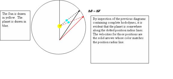
Next, we will see that the hododyne demonstrates how the velocity of the planet changes as the planet orbits the Sun. In the diagram below, the black arrow and red arrow correspond to the total velocity of the planet at two successive moments in time. We will now find that the arc of the circle between the tip of the red arrow and the tip of the black arrow is representative of the angle through which the planet on successive dotted lines travels in relation to the Sun and is also representative of the change in velocity of the planet as it moves through that angle.

 Momentarily, refer back to the previous diagram with the two representative hododyne positions displayed and recall that it was stated that segment CB represents the total speed and direction of the planet at any instant. From one orbital position to the next, the segment CB, representing total velocity, changes its size and orientation. In the figure above, CB is not labeled but is represented by the red solid line and then an instant later by the black solid line. This allows us to examine segment CB for two consecutive instants in time. Let’s pause to fill in some knowledge about vector arrows. If we place the tails of two vector arrows together, as we have done with the black and red vectors whose tails meet (at a point representing the empty focus of the ellipse as can be seen in the previous hodograph diagram with letter labels), then the change in velocity is determined by drawing a vector arrow from the tip of the initial velocity vector arrow to the tip of the final velocity vector arrow. In accordance with the rules for addition of vectors, we could draw a connecting line from the tip of the red velocity vector arrow to the tip of the black velocity arrow to represent the change in velocity. If the planet were traveling counter clockwise the velocity change arrow would point from the tip of the red arrow to the tip of the black arrow. Referring back to the hodograph with labels, the line segment AB contains the planet at point G and ends on the circle at point B. The line segment CB represents total velocity and also ends on the circle at point B. The change in velocity, the vector arrow connecting line for consecutive CB velocity segment tips, will trace the hodograph’s circle as it is repeatedly drawn to connect subsequent CB segment tips as the planet orbits. Note that the arc of angle that the planet travels relative to the Sun can also be measured along the same hodograph circle since the radius direction to the Sun is given by the line segment AB (which contains the planet at point G) which ends at point B also on the hodograph circle. By inspection of the labeled hodograph it is evident during an orbit that since point B is shared by line segments CB and AB,for any amount of arc of the circle traveled by the radius line connecting the planet to the Sun, there is an equal amount of arc traced by the tips of the initial and final corresponding total velocity vector arrow segment CB.  The arc traveled by the planet’s angle and the arc traveled by the change in velocity are identical. Thus the change in angle of position relative to the Sun is proportional to the change in total velocity. Credit goes to Richard Feynman for finding this relationship between the angle swept and the change in velocity and to David L. Goodstein and Judith R. Goodstein for analyzing, clarifying, and publishing the derivation in their book Feynman’s Lost Lecture : The Motion of Planets Around the Sun. In fact, their book demonstrates how this relationship between change in total velocity and the angle swept by a planet proves that gravitational force is inversely proportional to the square of distance.

There are many other aspects of orbits to describe using the approach of Orbits Explained. For example, we can show that, for every position along an orbital path, a planet has the same speed toward the Sun as it does 180 degrees away. This phenomenon can be a philosophical explanation for why planets stay in their stable orbits. We can also apply our methods and diagrams to compare orbits of differing sizes around the same Sun. In order to do this we employ a novel method of finding ways to scale hododyne diagrams of different size orbits. We can also use our methods to find formulae for characteristics of orbits such as the escape velocity of a planet and the Energy Equation of a planet. These topics are fully detailed in the book Orbits Explained. Other topics include thoughts on Bertram’s Theorem regarding the only possible orbital shapes, Hooke’s Law of Force, areal velocity, and the special positions of planets when they are at the tip of a semiminor axis of an ellipse or the tip of a semilatus rectum of an ellipse.

For those interested, the book can be purchased on the Amazon website by clicking here.

-David S. Marlin

 Los Angeles